Advanced Moving Average Variants
The SMA and EMA from Lesson 30 are the foundational variants. The advanced variants exist because traders identified specific limitations of the basics and developed mathematical modifications to address them — each a specific answer to a specific problem.
- Define WMA, DEMA, TEMA, HMA, KAMA, TMA, DMA, Median Average, VWMA, and Rainbow Average
- Calculate a weighted moving average (WMA) by hand from given price data
- Explain why the DEMA and TEMA reduce lag compared to the EMA, and what trade-off they create
- Describe how the Hull Moving Average achieves low lag while maintaining smoothness
- Explain the KAMA's adaptation mechanism and when adaptation is most valuable
- Choose the appropriate variant for a given trading application using the comparative framework
Why the Variants Exist
The simple moving average and exponential moving average from Lesson 30 are the foundational variants that everything else in the moving average family builds from. The advanced variants exist because traders working with moving averages identified specific limitations of the basic SMA and EMA and developed mathematical modifications to address those limitations. Each variant is a specific answer to a specific problem.
The most important problem the variants try to solve is lag. Both the SMA and the EMA lag price action — they can only reflect changes after they've happened. The lag is fundamental to how derivative calculations work (you can't average data that doesn't exist yet), but it creates real practical problems. A trader using a 50-period SMA to identify trend changes catches those changes well after they've started, by which point the easy gains are gone and the risk-reward has deteriorated. If a trader could reduce the lag without sacrificing too much smoothing, the moving average would become more useful for timing decisions.
Most of the advanced variants are attempts to reduce lag through various mathematical tricks. Some weight recent prices even more heavily than the EMA does. Some apply smoothing functions on top of the basic calculation. Some adapt their behavior to current market volatility. Some use higher-order mathematical operations to reduce lag while preserving smoothness. Each variant has trade-offs — reducing lag usually increases noise sensitivity, and increasing smoothness usually increases lag — but the variants offer different points on this spectrum that suit different trading styles and applications.
This lesson covers the major advanced variants together rather than giving each its own lesson because the underlying conceptual material from Lesson 30 transfers to all of them. Readers don't need to relearn what a moving average is or what its slope means; they need to understand what each variant does differently and when those differences matter. The lesson is structured as a comparative treatment so readers can see how the variants relate to each other and to the SMA and EMA baselines.
Vocabulary
- Weighted moving average (WMA) — A moving average where each bar in the window is multiplied by a weight factor, with weights increasing linearly toward the most recent bar. The weights are typically the bar's position in the window — for a 5-period WMA, the most recent bar gets weight 5, the next gets weight 4, then 3, 2, and 1 for the oldest bar. The weighted prices are summed and divided by the sum of the weights. Sits between SMA and EMA in responsiveness.
- Double exponential moving average (DEMA) — A moving average designed to reduce the lag of a standard EMA by applying a specific mathematical formula that effectively projects the EMA forward. Calculated as twice the EMA minus the EMA of the EMA. Responds notably faster than a standard EMA of the same period.
- Triple exponential moving average (TEMA) — Further reduces lag through a more complex formula involving three layers of exponential moving averages. Calculated as three times the EMA minus three times the EMA of the EMA plus the EMA of the EMA of the EMA. Responds even faster than DEMA but with more noise sensitivity.
- Hull moving average (HMA) — Developed by Alan Hull in 2005 specifically to dramatically reduce lag while maintaining smoothness. Uses a combination of weighted moving averages and a square-root smoothing step. Considered by many traders to be the best variant for combining responsiveness with smoothness, though at the cost of mathematical complexity.
- Kaufman adaptive moving average (KAMA) — Developed by Perry Kaufman. Adapts its smoothing constant based on the efficiency of recent price movement — when price is trending efficiently, KAMA responds faster; when price is choppy, KAMA smooths more aggressively. Designed to filter noise during ranging markets while staying responsive during trending markets.
- Adaptive moving average (in thinkorswim, MovAvgAdaptive) — A general category of moving averages that adjust their parameters based on market conditions. KAMA is the most common adaptive variant, but several others exist with different adaptation methods.
- Variable moving average (VMA) — Another adaptive moving average that adjusts its smoothing based on volatility measurements. Distinct from KAMA in its specific adaptation methodology but conceptually similar.
- Triangular moving average (TMA) — A double-smoothed moving average that applies SMA twice. Produces a smoother line than a single SMA but with more lag. Useful when extra smoothing is desired and lag is less important.
- Displaced moving average (DMA) — Any standard moving average shifted forward or backward in time using the displacement setting from Lesson 30. Same calculation as the underlying moving average, just positioned differently on the chart. Used to align moving averages with specific bar counts for analytical purposes.
- Median average — Uses the median price of each bar (typically calculated as (high + low) / 2) instead of the closing price as the input to the moving average. Less affected by gaps and outlier closes but loses the closing-price information that most moving averages rely on.
- Volume-weighted moving average (VWMA) — Weights each bar in the window by its volume rather than by position. Bars with heavy volume get more influence on the moving average than bars with light volume. Conceptually related to VWAP (which we'll cover in detail in a later lesson) but applied as a moving average across the chart's period rather than reset daily like VWAP.
- Rainbow average — A visualization technique that displays multiple moving averages of different periods simultaneously, typically with colors that create a rainbow-like effect. Used to see trend structure at multiple timeframes simultaneously on a single chart. The underlying moving averages are usually standard SMAs.
- Smoothing constant — The mathematical parameter that determines how much weight recent data gets versus older data in moving averages that use exponential weighting. The EMA's smoothing constant K is the canonical example; other variants have their own smoothing parameters with different formulas.
- Order of smoothing — How many times a smoothing function is applied within a moving average's calculation. SMA is first-order; DEMA effectively uses second-order smoothing; TEMA uses third-order. Higher orders generally reduce lag at the cost of mathematical complexity and noise sensitivity.
- Adaptation efficiency — A measure used by KAMA and other adaptive moving averages to quantify how directional recent price movement has been. High efficiency means price moved in a relatively straight line; low efficiency means price wandered substantially. The efficiency value drives how the moving average adapts.
The Weighted Moving Average (WMA)
The WMA addresses the SMA's main limitation — equal weighting across all bars — by introducing linear weighting that emphasizes recent bars. The calculation is more complex than the SMA but simpler than the EMA.
WMA Formula
WMA = (P₁ × n + P₂ × (n−1) + P₃ × (n−2) + ... + Pₙ × 1) / (n + (n−1) + (n−2) + ... + 1)
Where P₁ is the most recent price (gets the highest weight), Pₙ is the oldest price (gets weight of 1), and n is the period length. The denominator simplifies to n × (n+1) / 2 — the sum of the first n positive integers.
Working through an example. For a 5-period WMA with closing prices of 10, 11, 12, 11, and 13 (where 13 is the most recent), the calculation is: Numerator = (13 × 5) + (11 × 4) + (12 × 3) + (11 × 2) + (10 × 1) = 65 + 44 + 36 + 22 + 10 = 177. Denominator = 5 + 4 + 3 + 2 + 1 = 15. WMA = 177 / 15 = 11.8. Compare this to the SMA of the same data, which calculated to 11.4. The WMA is 11.8 — slightly higher, because the most recent price (13) gets weight 5 while the oldest price (10) gets weight 1. The WMA emphasizes the recent rally more than the SMA does.
What the math reveals about WMA behavior. The linear weighting puts the WMA between the SMA and the EMA in terms of responsiveness. It responds faster than the SMA because recent bars matter more, but it responds slower than the EMA because the weight reduction is linear (going from 5 to 1) rather than exponential (going from a high smoothing constant to a very low one as you move backward through time).
When to use the WMA. The WMA is useful when traders want more responsiveness than the SMA but less than the EMA. In practice, the difference between WMA and EMA is small enough that most traders simply use the EMA. The WMA exists in the platform for traders who specifically want linear weighting rather than exponential weighting, but the practical applications are limited.
The Double Exponential Moving Average (DEMA)
The DEMA was developed by Patrick Mulloy in 1994 specifically to reduce the lag of standard EMAs. The approach is mathematically clever: take the EMA, then take the EMA of the EMA, then combine them in a way that effectively cancels out much of the original EMA's lag.
DEMA Formula
DEMA = (2 × EMA) − EMA(EMA)
Where EMA is the standard exponential moving average of the price, and EMA(EMA) is the EMA of that EMA — essentially smoothing the EMA itself.
Why this reduces lag. The reasoning is that the EMA of the EMA represents a "doubly smoothed" version of price, which lags more than the original EMA. Subtracting it from twice the original EMA produces a line that follows price closer than either the EMA or its smoothed version. The result is a moving average that responds notably faster to price changes while maintaining most of the smoothness of the underlying EMA.
Working through an example. Assume the 20-period EMA is 100.00 and the 20-period EMA of that EMA is 99.50 (slightly lower because of the additional smoothing lag). The DEMA would be: DEMA = (2 × 100.00) − 99.50 = 200.00 − 99.50 = 100.50. The DEMA reads 100.50, ahead of both the EMA (100.00) and the EMA of the EMA (99.50). When price is trending up, the DEMA leads the EMA toward the new direction.
What the math reveals about DEMA behavior. The lag reduction is real and significant — a 20-period DEMA often responds to price changes nearly as quickly as a 10-period EMA, but with more smoothing. This makes the DEMA useful for traders who want EMA-style smoothing with reduced lag. The trade-off is increased complexity: the DEMA's behavior is harder to predict intuitively than a simple EMA because two layers of calculation are involved.
When to use the DEMA. When the standard EMA's lag is causing problems — entries happening too late, exits happening too late — the DEMA offers an alternative with reduced lag. The DEMA is particularly useful on shorter timeframes where lag matters more, though it can be used on any timeframe.
The Triple Exponential Moving Average (TEMA)
The TEMA extends Mulloy's lag-reduction approach one step further by using three layers of EMA calculation instead of two. The formula is more complex but the reasoning is the same: cancel out more of the lag while maintaining smoothness.
TEMA Formula
TEMA = (3 × EMA) − (3 × EMA(EMA)) + EMA(EMA(EMA))
Three layers of EMA combined in a way that further reduces lag beyond what DEMA achieves.
What this means practically. The TEMA responds even faster than the DEMA, but with increased noise sensitivity. The additional mathematical complexity that reduces lag also makes the TEMA more responsive to short-term price oscillations that don't represent meaningful trend changes. Traders who use the TEMA need to accept this trade-off — they get faster signals but also more false signals.
When to use the TEMA. The TEMA is useful when even the DEMA isn't responsive enough for the trader's purposes. In practice, traders working on short timeframes (intraday, scalping) sometimes prefer the TEMA for its fast response. Traders on longer timeframes (daily, weekly) usually find the DEMA's noise filtering more useful than the TEMA's additional responsiveness.
QuantifiedStrategies' research on the triple exponential moving average (TEMA) found that triple exponential moving average strategies do work, with backtests showing that the TEMA can be used profitably for long-term trend-following strategies on stocks. The TEMA is a trend-following indicator formulated by creating multiple exponential moving averages of the original EMA to reduce some of the lag.
The Hull Moving Average (HMA)
The Hull moving average was developed by Alan Hull in 2005 and represents one of the more mathematically sophisticated approaches to combining responsiveness with smoothness. The HMA uses a specific combination of weighted moving averages that produces remarkable lag reduction without sacrificing too much smoothness.
HMA Formula
HMA = WMA(2 × WMA(n/2) − WMA(n), √n)
Where n is the period length, WMA(n) is a weighted moving average with period n, WMA(n/2) is a weighted moving average with period n divided by 2, and √n is the square root of n rounded to the nearest integer.
- Calculate a WMA with period n/2 (a shorter, more responsive WMA)
- Calculate a WMA with period n (the standard period WMA)
- Take twice the first WMA minus the second WMA — this creates a line that responds quickly
- Smooth that result with a WMA of period √n to reduce noise without adding much lag back
Working through the conceptual logic. The first step (the difference between a short WMA and a longer WMA) creates a fast-responding signal that's also noisy. The second step (smoothing with a √n WMA) reduces the noise while adding minimal lag because √n is much smaller than n. The result is a moving average that responds very quickly to genuine price changes while filtering out short-term noise.
What the math reveals about HMA behavior. The HMA often responds to price changes faster than even short-period EMAs, but with smoothness comparable to longer-period SMAs. This combination is what makes the HMA popular with traders who want a single moving average that does the work of multiple traditional moving averages.
When to use the HMA. The HMA is increasingly popular among traders who find the standard SMA and EMA either too laggy or too noisy. It serves as a kind of compromise that combines the best features of both. Liberated Stock Trader's comparative testing across 43,770 trades found that at moving average settings of 50, 100, and 200, it is better to use the Hull moving average, which has win rates of 27%, 10%, and 17% respectively — outperforming SMA, EMA, and WMA at these longer settings.
The Kaufman Adaptive Moving Average (KAMA)
The KAMA represents a different approach to moving average improvement than the lag-reduction methods above. Instead of using fixed mathematics to reduce lag, the KAMA adapts its behavior based on current market conditions.
The conceptual approach. Perry Kaufman observed that fixed-parameter moving averages have an inherent problem: any single smoothing setting works well in some market conditions and poorly in others. A fast-responding moving average works well in trending markets but produces excessive false signals in ranging markets. A slow-responding moving average filters noise well in ranging markets but catches trend changes too late. Kaufman's solution was to create a moving average that uses different smoothing depending on what the market is currently doing.
How the adaptation works. The KAMA calculates an "efficiency ratio" for each bar that measures how directional recent price movement has been. The efficiency ratio is calculated as the net price change over a lookback period divided by the sum of absolute price changes within that period. When price moves in a straight line, the efficiency ratio is high (near 1). When price oscillates substantially with little net progress, the efficiency ratio is low (near 0).
The KAMA then uses this efficiency ratio to determine how aggressive its smoothing should be. High efficiency (trending market) means the KAMA uses a smoothing constant close to a fast EMA. Low efficiency (ranging market) means the KAMA uses a smoothing constant close to a slow EMA. The result is a moving average that responds quickly when responsiveness is valuable (during trends) and smooths heavily when smoothing is valuable (during ranges).
KAMA Formula (simplified)
KAMA today = KAMA yesterday + SC × (Price today − KAMA yesterday)
SC is the smoothing constant that varies based on the efficiency ratio. The SC formula combines the efficiency ratio with constants that define the fastest and slowest possible smoothing the KAMA will use.
What the math reveals about KAMA behavior. During strong trends, the KAMA behaves like a fast EMA, catching trend changes quickly. During ranging markets, the KAMA behaves like a slow SMA, filtering out the choppy oscillations. The adaptation happens automatically based on the market conditions — the trader doesn't need to manually adjust settings.
When to use the KAMA. The KAMA is particularly valuable for traders who trade multiple market conditions and don't want to manually adjust their moving average settings. It's also useful as a filter for distinguishing trending from ranging markets — when the KAMA is responding quickly to price changes, the market is trending; when it's smoothing heavily, the market is ranging.
The Triangular Moving Average (TMA)
The TMA is a double-smoothed moving average that applies the SMA calculation twice. The result is a very smooth moving average with more lag than a standard SMA.
TMA Formula
TMA = SMA(SMA(price, n), n)
Calculate the standard SMA first, then take the SMA of that SMA. The result is a doubly-smoothed line.
What this produces. The TMA's defining characteristic is its smoothness — it shows only major directional movements and filters out almost all short-term noise. The trade-off is significant lag, often greater than a single SMA of double the period.
When to use the TMA. The TMA is useful when extra smoothness is desired and timing isn't critical. Some traders use the TMA for longer-term trend identification where the smoothness reveals the underlying trend more clearly than less-smoothed alternatives. The TMA is less commonly used than other variants because most traders prefer faster responses, but it has its place for specific applications.
The Displaced Moving Average (DMA)
The DMA isn't a new calculation — it's any standard moving average shifted forward or backward in time using the displacement setting. The underlying moving average can be SMA, EMA, or any other variant; the displacement just changes where the moving average appears on the chart.
Why displacement matters. When a moving average is displaced forward (into the future on the chart), the current value of the moving average is positioned ahead of the bars it was calculated from. This is sometimes useful for analyzing how price might interact with the moving average in future bars. When displaced backward, the moving average is positioned behind the bars it was calculated from, which can help identify historical pivot points where the moving average aligned with structural levels.
Practical applications. Most traders don't use displacement at all and leave the setting at zero. The traders who use displacement are typically doing specialized analysis — often related to Bill Williams' Alligator indicator or similar systems that specifically use displaced moving averages. For general-purpose use, displacement adds complexity without adding much analytical value.
The Median Average
The median average uses the median price of each bar instead of the closing price as the input to a standard moving average calculation. The median price is typically defined as (high + low) / 2 — the midpoint of each bar's range.
Why use median prices. Closing prices can be affected by end-of-session activity that doesn't reflect the bar's overall character — large orders placed at the close, end-of-day fund rebalancing, or news that affects only the final minutes. The median price represents the middle of the bar's range and is less affected by these end-of-period influences.
Trade-offs. The median average is more stable than the closing-price moving average in some respects but loses the closing-price information that most other analysis uses. Most technical analysis assumes closing prices are the most important values for each bar because they represent the day's final consensus. Using median prices breaks this consistency and can produce different signals than closing-price-based moving averages.
When to use. The median average has limited mainstream adoption. Traders who specifically prefer median prices for their analysis use it; most traders stick with closing-price moving averages.
The Volume-Weighted Moving Average (VWMA)
The VWMA weights each bar in the window by its volume rather than by position. Bars with heavy volume get more influence on the moving average than bars with light volume.
VWMA Formula
VWMA = Σ(Price × Volume) / Σ(Volume)
Where the sum runs across the bars in the window. Each bar's price is multiplied by its volume, the products are summed, and the total is divided by the sum of volumes.
Why volume weighting matters. A bar with heavy volume represents more market participation than a bar with light volume — more traders contributed to the price action, which arguably makes the price more meaningful as a reference. By weighting moving averages by volume, the VWMA emphasizes the price levels where the most trading actually occurred.
Relationship to VWAP. VWMA is conceptually related to VWAP (volume-weighted average price), which we'll cover in detail in a later lesson. The main difference is that VWAP typically resets at the start of each trading session and accumulates throughout the day, while VWMA is a continuously calculated moving average across the chart's period. VWMA is useful for any timeframe; VWAP is primarily a day-trading tool.
When to use the VWMA. Traders who believe volume should weight their analysis use VWMA instead of or alongside standard moving averages. The VWMA tends to differ most from standard moving averages during periods of high-volume activity (earnings, news events) when the volume weighting changes which bars matter most.
The Rainbow Average
The rainbow average isn't a single moving average — it's a visualization technique that displays multiple moving averages of different periods simultaneously, typically with colors that create a rainbow-like effect from short periods to long periods.
How it works. A typical rainbow average might display 10 SMAs of periods from 2 to 200, with each SMA colored differently. The result is a band of lines on the chart showing the moving averages at progressively longer timeframes.
What the rainbow shows. When all the moving averages are stacked in order (short periods above long periods in an uptrend, short periods below long periods in a downtrend), the trend is structurally clean. When the moving averages tangle together with shorter periods crossing through longer periods, the trend is structurally messy and likely transitional.
When to use. The rainbow average is useful for visualizing trend structure quickly. Some traders find it helpful for identifying when trends are healthy versus when they're approaching exhaustion. Most traders don't use it for entry timing because the visual complexity makes precise signal identification difficult.
Comparing the Variants: When Each Is Appropriate
Now that the individual variants have been covered, the practical question for readers is: which variant should they actually use? The honest answer is that for most use cases, the choice doesn't matter much — the differences between variants are smaller than the differences in how traders apply them. But for specific applications, the choice does matter.
- For straightforward trend identification on daily charts: SMA or EMA. The advanced variants don't add enough value to justify the added complexity for this use case. Stick with the canonical periods (20, 50, 200) and the standard SMA or EMA.
- For shorter-term trading where lag matters: DEMA or HMA. The lag reduction these variants provide can genuinely improve entry timing on shorter timeframes. The HMA is more popular but the DEMA is simpler to understand.
- For adapting to changing market conditions: KAMA. The automatic adaptation to trending versus ranging markets makes the KAMA valuable when the trader is working across multiple market regimes.
- For very smooth trend identification: TMA or longer-period SMAs. When smoothness matters more than timing, the doubly-smoothed TMA or longer-period basic moving averages serve well.
- For volume-aware analysis: VWMA. When the trader specifically wants volume to weight their moving average analysis, the VWMA is the right tool.
- For specialized applications: The remaining variants (median average, rainbow, displaced moving averages) serve specific niche applications and shouldn't be used without specific reasons to choose them.
Start with SMA and EMA. Get genuinely comfortable with them. If you encounter specific problems that the standard moving averages don't solve well, then explore the variants that address those specific problems. Don't pile on advanced variants because they sound sophisticated — the sophistication doesn't help if the underlying analysis isn't sound.
Pattern Statistics and Sources
The published research on moving average variants is less extensive than the research on basic SMA and EMA, partly because variants are less widely used and partly because the differences between variants are often smaller than the methodological variations across studies. But some general findings exist.
Liberated Stock Trader's comparative testing across 43,770 trades found that at the 20-period setting, SMA and EMA produced the best results with a 23% win rate. At settings of 50, 100, and 200, the Hull moving average outperformed other variants with win rates of 27%, 10%, and 17%. This suggests the HMA's lag reduction is most valuable at longer periods where SMA and EMA lag would be most significant.
QuantifiedStrategies' research on TEMA found that triple exponential moving average strategies work for long-term trend-following on stocks. The TEMA can be used profitably with proper application, though the research focuses on trend-following applications rather than crossover signals.
The variants share the same fundamental limitation as basic moving averages: they perform poorly as standalone trade signals and substantially better as components within multi-factor analysis. Switching from SMA to HMA doesn't transform a poor strategy into a good one — the underlying issue is using moving averages alone rather than integrating them with price action analysis.
- liberatedstocktrader.com — comparative testing across multiple moving average variants with specific reliability figures at different settings
- quantifiedstrategies.com — research on specific variants including TEMA, DEMA, and HMA applications
- thinkorswim.com documentation — official Schwab platform documentation on each variant's calculation methodology
- The original publications by the variant developers (Mulloy on DEMA and TEMA, Hull on HMA, Kaufman on KAMA) — for traders who want to understand the mathematical reasoning behind each variant directly from the source
- Academic literature via Google Scholar — search "adaptive moving average," "Hull moving average," "moving average comparison"
Common Student Mistakes with Advanced Moving Average Variants
- Choosing variants based on sophistication rather than purpose. The variants exist because they solve specific problems. A trader who chooses DEMA over EMA because DEMA "sounds more advanced" is making a choice without understanding what problem they're solving. The correct selection process is: identify the specific limitation of the basic moving average you're using, then choose the variant that addresses that limitation.
- Switching variants when results disappoint. When trades aren't working, the temptation is to assume the moving average is the problem and switch to a different variant. Usually the problem isn't the moving average — it's the underlying strategy or execution. Switching variants without diagnosing the actual issue produces variant-shopping behavior that wastes time without improving results.
- Using too many variants simultaneously. Adding SMA, EMA, DEMA, TEMA, and HMA all to the same chart produces visual chaos without analytical benefit. The variants are showing the same underlying price data with slightly different smoothing approaches. Pick one variant for each role you need a moving average to play (one for trend identification, one for entry timing if you use a second one) and ignore the others.
- Treating variant differences as larger than they are. The differences between SMA and EMA, between EMA and DEMA, between DEMA and HMA are real but small in most market conditions. Most of the time, a 20-period SMA and a 20-period EMA produce similar signals. The variants matter at the margins — in specific market conditions where their unique characteristics provide advantages — but they don't transform the underlying analysis.
- Ignoring the increased complexity cost. Every variant beyond SMA and EMA adds cognitive overhead. The trader needs to understand what the variant is doing, how it differs from alternatives, and when its specific characteristics matter. This cognitive cost is real and not free. For most traders, the simplicity of SMA and EMA is worth more than the marginal improvements the variants provide.
- Using KAMA and other adaptive variants without understanding the adaptation. When KAMA's behavior changes (sometimes smoothing heavily, sometimes responding quickly), traders who don't understand the adaptation can find the changes confusing or unpredictable. Adaptive variants require more conceptual investment than fixed-parameter variants. Traders who use them without making that investment often abandon them after getting confused by their behavior.
Reading Variant Comparisons on a Chart
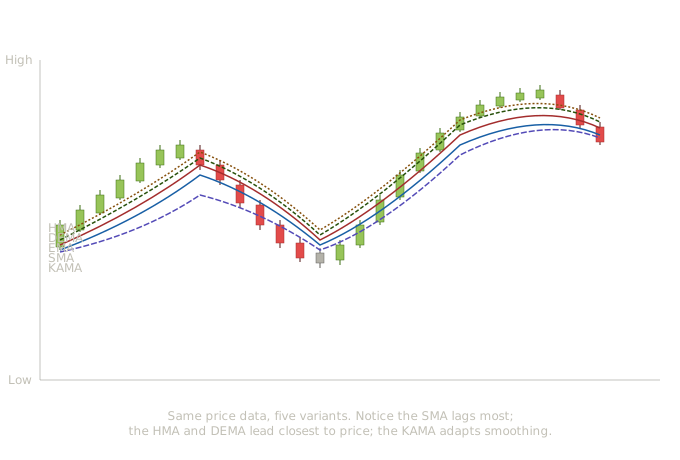
Five 20-period moving average variants on the same price data — SMA, EMA, DEMA, HMA, and KAMA showing different response speeds to the same price action
Reading the Variant Comparison Through Both Layers
The chart shows the same price data with five different 20-period moving averages overlaid: SMA, EMA, DEMA, HMA, and KAMA. Looking at how each line responds to the same price action teaches readers what the mathematical differences actually mean in practice.
The early uptrend (candles 1-7). Seven bullish candles establish the initial direction. Notice that all five moving averages slope upward, but they don't slope upward at the same rate. The HMA pulls upward first, followed closely by the DEMA, then the EMA, then the SMA, with the KAMA tracking somewhere between the EMA and the SMA. This is exactly what the math from the lesson predicts: the HMA's lag-reduction formula pulls it closest to current price, the DEMA's double-EMA construction puts it second, the EMA is third because of its exponential weighting, the SMA is fourth because of its equal weighting, and the KAMA is positioned based on how it's adapting to current conditions.
The peak and reversal (candles 7-9). Price reaches a high and begins reversing. Watch how each moving average responds to the reversal. The HMA reverses direction almost immediately as the bearish candles begin. The DEMA reverses shortly after. The EMA takes longer to reverse. The SMA reverses last and most slowly. The KAMA reverses at a pace determined by its current adaptation — if the market has been trending (high efficiency), it reverses relatively quickly; if the market has been choppy (low efficiency), it reverses slowly.
This is the lag trade-off in visible form. The HMA's fast response means it caught the reversal earlier — but it also means the HMA would respond just as quickly to a brief pullback that doesn't actually reverse the trend, producing more false signals in choppy markets. The SMA's slow response means it confirms reversals later — but it also means it filters out false reversals that don't sustain.
The decline (candles 8-13). Six bearish candles drive price down. The moving averages spread visibly during the decline — the faster-responding variants (HMA, DEMA) pull downward more aggressively, while the slower variants (SMA, KAMA when adapting to choppiness) lag behind. The spreading between variants is itself informative: when the spread is large, the market is moving directionally; when the spread is small (the variants converge), the market is consolidating.
The small-body bottom (candle 14). A small-body candle marks the decline's bottom. This is the kind of indecision candle from Lesson 4 that often appears at turning points. None of the moving averages anticipate this turn — they're all still sloping downward when the candle forms because each is showing past directional movement, not future direction. This is the fundamental limitation we discussed in Lesson 29: moving averages can only summarize what already happened, never predict what's about to happen.
The recovery rally (candles 15-23). Nine bullish candles drive price up substantially. Watch how the moving averages reverse their slopes at different rates. The HMA flips bullish first; the DEMA follows; the EMA comes next; the SMA reverses last. By the time all five moving averages are sloping upward, the rally is well established. A trader watching the HMA caught the turn earliest; a trader watching the SMA caught the turn latest but with the most confirmation.
The continued rally (candles 24-26). Three more bullish candles continue the move. The moving averages are now all sloping upward at similar rates. This is what a confirmed uptrend looks like across multiple moving average variants — they all agree on the direction, and the spread between them is moderate (not the wide spread of acceleration, not the convergence of consolidation).
The reversal at the top (candles 27-29). Three bearish candles begin a new decline. The faster variants respond first; the slower variants lag. The pattern repeats — fast variants catch turns earlier with more noise; slow variants catch turns later with more confirmation.
What This Comparison Teaches Together
The chart demonstrates the central trade-off that defines moving average variant selection: responsiveness versus smoothness. Every variant sits somewhere on this spectrum, and the right choice depends on what the trader needs the moving average to do.
For early signal detection in clean trends: the HMA and DEMA are excellent. They catch directional changes faster than basic moving averages, which means earlier entries and exits. The cost is more false signals when markets are choppy because the same fast response triggers on noise.
For trend confirmation that filters noise: the SMA and TMA work well. They lag more, which means later signals, but the lag also filters out false signals from short-term oscillations. The cost is missing the early portion of moves.
For automatic adaptation across market conditions: the KAMA shines. When markets are trending, it behaves like a fast variant. When markets are choppy, it behaves like a slow variant. The adaptation happens without the trader manually adjusting settings.
For most traders, the EMA is a reasonable default. It sits in the middle of the responsiveness-smoothness spectrum, has the most published research behind it, integrates with most other indicators that reference moving averages, and behaves predictably enough that traders can develop intuition for it.
The point isn't that one variant is best. The point is that each variant has characteristics that make it appropriate for different applications, and readers should choose deliberately based on what they need rather than randomly or based on marketing claims.
Making Trading Decisions with Variant Moving Averages in Real Time
The real-time decision-making walkthrough from Lesson 30 applies just as much when readers use advanced variants — possibly more, because the variants' specific characteristics create their own decision dynamics. Let's walk through what trading with different variants actually looks like at key moments on this chart.
A trader using the HMA would see the HMA already responding to the decline's slowdown — the HMA's slope is starting to flatten. The trader has an early hint that the decline may be ending, but it's just a hint. A trader using the SMA would see the SMA still sloping confidently downward — no hint yet that anything is changing. A reasonable decision varies by variant. The HMA user might take a small starter long position on the small-body candle, betting on the bottom forming. The SMA user might wait — their moving average isn't suggesting anything has changed yet. Both decisions are rational given the information each variant provides.
What happens next. The recovery rally develops over the following sessions. The HMA user who took the starter position is now profitable on their early entry. The SMA user who waited has not yet entered but is also not at a loss. Both traders are still positioned to participate in the rally, just from different cost bases.
A trader using the HMA sees the HMA already sloping firmly upward, providing dynamic support that price has tested and held. They might add to their long position with confidence. A trader using the SMA sees the SMA just beginning to slope upward — they might enter their initial position here, later than the HMA user but with stronger confirmation that the trend is real. The trade-offs in concrete form: the HMA user has been in the trade longer and with better cost basis. The SMA user has been in the trade for less time with worse cost basis but with more confirmation that the trade is working. Neither trader has made a bad decision; they've made different decisions reflecting their different tools.
A trader using the HMA sees the HMA already flattening — possibly an early warning of trend exhaustion. A trader using the SMA sees the SMA still sloping confidently upward — no warning yet. The HMA user might take profits or tighten stops based on the early warning. The SMA user has no reason yet to do anything — their tool is not signaling caution.
What happens next. The bearish candles develop and the rally ends. The HMA user who took early profits captured the move at its peak. The SMA user who held on watches profits erode as price declines. The HMA user looks brilliant in retrospect; the SMA user looks like they overheld.
But here's where the honest mindset from Lesson 30 matters. This same scenario played in the opposite direction would show the SMA user winning. In a healthy trend with a temporary pullback, the HMA would flatten warning the trader to exit, the trader would exit, and then price would continue higher leaving the early-exit trader on the sidelines. The SMA user who didn't get the early warning would still be in the trade and would capture the additional move.
Neither variant produces better outcomes consistently. They produce different outcomes in different market conditions. The HMA user wins when trends reverse cleanly and the warning was correct. The SMA user wins when warnings are false and trends continue. Over time, the results tend to be similar because each variant's strengths balance against its weaknesses.
The Mindset for Choosing Among Variants
The mindset work we introduced in Lesson 30 extends naturally to variant selection. The trader who switches variants every time their current variant produces a frustrating result is doing the same dysfunctional thing as the trader who second-guesses individual trades based on what happened after the exit. They're trying to optimize for outcomes that can't be optimized for.
Each variant has its inherent characteristics. The HMA catches turns earlier and produces more false signals. The SMA catches turns later and filters more false signals. Switching between them based on which one would have worked better on the last trade is exactly the wrong process. The right process is choosing a variant deliberately based on the trading style and market conditions, then accepting the variant's inherent trade-offs as part of how trading works.
Traders who can't accept the trade-offs end up variant-shopping — constantly switching between SMA, EMA, DEMA, TEMA, HMA, KAMA looking for the magic combination that produces only good signals. This combination doesn't exist. Every variant produces some good signals and some false signals because they're all mathematical transformations of the same price data, which is itself imperfect as a prediction tool.
The traders who succeed with variants are the ones who choose deliberately, accept the trade-offs, and focus on executing their chosen variant well rather than searching for a better one. The same principle that applied to executing trades imperfectly in Lesson 30 applies to choosing variants imperfectly here — you make the best decision you can with the information you have, accept that the decision wasn't perfect, and keep moving forward.
How This Lesson Connects to What Comes Next
Lesson 32 covers moving average crossovers — the golden cross, death cross, and the various automated crossover detection studies available in the platform. The crossover concept builds directly on the moving average understanding from Lessons 30 and 31. When two moving averages cross each other, the crossover represents a moment where the relationship between two different smoothing levels of the same price data has changed direction. Understanding what the crossover actually means requires understanding what each moving average represents — which is exactly the foundation Lessons 30 and 31 built.
The lessons after that move through moving average envelopes and Bollinger Bands (Lesson 33), then into the major momentum oscillators starting with RSI (Lesson 34), then MACD (Lesson 35), then the other momentum tools (Lesson 36). Each subsequent lesson assumes the moving average foundation from Lessons 30 and 31 because moving averages appear inside or alongside almost every other indicator in the platform.
By the time readers complete Lesson 32, they'll have a complete understanding of the moving average ecosystem: what moving averages are, how the variants differ, how crossovers work, and how the entire family fits within broader technical analysis. This foundation supports everything that comes after.
Key Takeaways
- Advanced MA variants exist primarily to reduce lag — each is a specific mathematical answer to the SMA/EMA's lag problem, with its own trade-offs
- WMA uses linear weighting (most recent bar gets highest weight); DEMA = 2×EMA − EMA(EMA); TEMA = 3×EMA − 3×EMA(EMA) + EMA(EMA(EMA))
- HMA achieves low lag and high smoothness through a four-step WMA combination; at periods of 50, 100, and 200 it outperforms SMA, EMA, and WMA in published research
- KAMA adapts its smoothing based on market efficiency — fast in trending markets (high efficiency ratio), slow in ranging markets (low efficiency ratio)
- The lag trade-off is unavoidable: faster response means more false signals; slower response means later signals. Choose deliberately based on trading style, not sophistication
- Variant-shopping — switching between moving average types based on which one would have worked better last time — is as destructive as second-guessing individual trade decisions
- For most use cases, SMA and EMA are sufficient. Explore advanced variants only when you've identified a specific limitation of the basics that a variant solves
Quiz — 3 Questions
Answer one at a timeThe DEMA is calculated as (2 × EMA) − EMA(EMA). If the 20-period EMA is 100.00 and the 20-period EMA of that EMA is 99.00, what is the DEMA, and why is it positioned differently from the EMA?
In this lesson
400 — Technical Indicators — Integration and Methodology